
In my previous post on convolutional neural networks we looked at how to implement a simple neural upscaling network in Vulkan compute. We’ve shown a very basic, naive kernel which ran much too slow for use in real-time applications. In this post we’ll look at some initial optimizations we could do to remedy this and get closer to our goal of running it at interactive speeds.
Where we left off
Our naïve kernel consists of 4 nested for-loops which are ran in parallel for each pixel. Simplified, it looks something like this:
for (uint co = 0; co < out_channels; ++co) {
    float sum = 0;
    for (uint ci = 0; ci < in_channels; ++ci) {
        for (int ky = 0; ky < kernel_size_y; ++ky) {
            for (int kx = 0; kx < kernel_size_x; ++kx) {
                uint3 input_pixel = uint3(
                    out_pixel.x + kx - kernel_size_x / 2,
                    out_pixel.y + ky - kernel_size_y / 2,
                    ci
                );

                sum += input_image[input_pixel] * weights[weight_index++];
            }
        }
    }

    output_image[uint3(out_pixel, co)] = sum + biases[co];
}On my RTX 500 Ada laptop GPU, this kernel takes 393ms to process a 1280x720p image using the upscaling network from the previous post. If we want to run this upscaling interactively at 30 frames per second we need to optimize this to run in about 33ms, 12 times at fast! That’s a long way to go, so let’s get started.
Vectorization
Our current kernel loads memory for one element at a time: one value from the input image and one weight. Practically every modern GPU has specialized instructions available for loading much more data in a single transaction. A good balance here would be to load 4 elements per thread, giving us a 16-byte transaction. This keeps register usage per thread still low, and allows us to use 4-element image formats to force 4 consecutive values in memory.
Our inner-most two loops iterate over the convolution kernel. This is either 5×5 (25 elements) or 3×3 (9 elements) in our network, which make it a poor fit to vectorize: both 25 or 9 elements don’t align well when working with 4 element batches. Instead, we can reorder our dimensions a bit and vectorize over the input channels instead. We’ll store 4 input channels consecutively per pixel, and also reorder the weights to have 4 channels consecutively before moving to the next pixel.
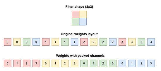
In our shader we can simply change their data types in the shader from float to float4. On the host side the input/output images should be changed from VK_FORMAT_R32_SFLOAT to VK_FORMAT_R32G32B32A32_SFLOAT.
The input image for the first pass is just one channel, so it doesn’t need reordering. The weights must be transformed in order to get 4 input channels consecutively. The C++ code for this relatively simple, but there’s an example here.
Then finally we also have to make some changes to our kernel. We can evaluate 4 input channels at once, but we also must evaluate 4 output channels before we can write back the result. To facilitate this, we move the inner loops into a separate conv() function which evaluates the result for a single output channel. We then have the outer loop over output channels call this method 4 times before writing the output image:
float conv(uint2 out_pixel, uint co)
{
    float4 sum = 0;
    uint weight_index = co * in_channel_blocks * kernel_size_y * kernel_size_x;
    for (uint ci = 0; ci < in_channel_blocks; ++ci) {
        for (int ky = 0; ky < kernel_size_y; ++ky) {
            for (int kx = 0; kx < kernel_size_x; ++kx) {
                uint3 input_pixel = uint3(
                    out_pixel.x + kx - kernel_size_x / 2,
                    out_pixel.y + ky - kernel_size_y / 2,
                    ci
                );

                // Vectorized load operations
                sum += input_image[input_pixel] * weights[weight_index++];
            }
        }
    }

    // Add all partial sums and the bias
    return sum.x + sum.y + sum.z + sum.w + biases[co];
}

void main(uint3 dispatch_thread_id : SV_DispatchThreadID) {
    const uint2 out_pixel = dispatch_thread_id.xy;

    for (uint co = 0; co < out_channel_blocks; ++co) {
        // Evaluate 4 consecutive output channels into a packed result
        float4 result;
        result.x = conv(out_pixel, co * 4 + 0);
        result.y = conv(out_pixel, co * 4 + 1);
        result.z = conv(out_pixel, co * 4 + 2);
        result.w = conv(out_pixel, co * 4 + 3);

        // Vectorized store operation
        output_image[uint3(out_pixel, co)] = apply_relu ? relu(result) : result;
    }
}We’ll also need some other minor changes, such as updating the relu() function to take a float4 and update the encode/decode kernels to handle the packed values. We also pass in new spec constants for the input and output channel block count, which is just the channel count divided by 4, rounded up. Those additions are trivial and left out here for brevity.
Now what does this gain us? Our runtime decreases to 259ms. Not bad!
| Naïve | 393ms |
| Packed vectors | 259ms |
| Target | 33ms |
Reducing memory traffic
Our previous step increased the efficiency of our memory access. But we are still accessing the same amount of memory over the course of our entire convolution operation. This amount is actually quite hefty. If you recall from the previous article, our network has 4 layers. The layers read from input images with 1, 64, 64 and 32 channels respectively. For the second layer, this input image has a size of 1280 (width in pixels) x 720 (height in pixels) x 64 (channels) x 4 (bytes per pixel) = 225 MB.
But this input isn’t loaded once. Every thread loads the same input image multiple times: once per output channel. So for the second pass this becomes 225 MB x 64 (output channels) = 14,400 MB of data transferred for just this convolution pass.
The table below shows the total memory transferred for each layer.
| # | Channels in | Channels out | Kernel | Input image size | Total input reads |
| 1 | 1 (4) | 64 | 5×5 | 14 MB | 896 MB |
| 2 | 64 | 64 | 3×3 | 225 MB | 14,400 MB |
| 3 | 64 | 32 | 3×3 | 225 MB | 7,200 MB |
| 4 | 32 | 9 (12) | 3×3 | 112.5 MB | 1350 MB |
| 576.5 MB | 23,846 MB |
(In practice it might even be worse. Every thread doesn’t load just a single pixel of the input image, but rather a small tile equal to its convolution kernel size. However, for simplicity we’ll assume that most of those reads will come from L1/L2 cache. This isn’t entirely accurate. But more about that later!)
So we need to load roughly 24 GB of input data for our entire convolution network. Looking at the specs for my RTX 500 again, NVIDIA reports it has a memory bandwidth (VRAM) of 128 GB/s. Just loading this input data for our convolution network would take 24 GB / 128 GB/s ≈ 0.188s or 188ms to run.
And that is excluding loading the weights, performing convolution calculations and storing the output image. So clearly this won’t work if we want to get down to 33ms. Luckily there’s an easy improvement we can do to reduce the amount of data our model needs: lowering our data precision.
We currently store both our data and model weights in 32-bit floating point numbers (fp32). When running inference in neural networks it is very typical to just use 16-bit floats (fp16) instead, which in practice results in negligible quality-loss.
This is a very simple change, we change our shader types from float4 to float16_t4, and update our images to use VK_FORMAT_R16G16B16A16_SFLOAT. And before we upload our weights and biases we convert them to fp16 using this rather dense C++ function (credit to Moritz Lehmann et al. [1]):
static uint16_t float_to_half(const float x) {
    const uint32_t b = std::bit_cast<uint32_t>(x) + 0x00001000;
    const uint32_t e = (b & 0x7F800000) >> 23;

    const uint32_t m = b & 0x007FFFFF;

    return static_cast<uint16_t>(
        (b & 0x80000000) >> 16 | (e > 112) * ((((e - 112) << 10) & 0x7C00) | m >> 13)
        | ((e < 113) & (e > 101)) * ((((0x007FF000 + m) >> (125 - e)) + 1) >> 1)
        | (e > 143) * 0x7FFF
    );
}This gives us a substantial speed-up, reducing the runtime to 124ms! As our performance was heavily limited by memory traffic, it makes sense that halving memory traffic would see about a 50% speed up. The actual results are even a bit better, which is likely the compounding effect of less data loaded from global memory, and smaller data allowing more re-use of loaded data from L1 and L2 caches.
| Naïve | 393ms |
| Packed vectors | 259ms |
| Conversion to fp16 | 124ms |
| Target | 33ms |
Before we move on we must note that this change technically changes the behaviour. We didn’t measure exactly what the resulting quality drop from reducing precision is. There are many other alternative datatypes we could potentially use, such as using the bfloat16 (bf16) datatype which has higher dynamic range than fp16, or even the fp8 datatype where it is supported. We could also use different datatypes for the image data and for the weights.
Nevertheless, to the naked eye the result with fp16 is practically indistinguishable from fp32 and fp16 is much better supported than the alternatives, so we’ll stick with that.
A profiling intermezzo
We made some nice improvements, but before we move on it would be good to know what is currently limiting our kernel’s performance. As I have a NVIDIA GPU, I’ll use Nsight Graphics to profile the Vulkan Compute kernel dispatch (On AMD GPUs you can use the Radeon GPU Profiler).
One of the most important metrics to look at is how much of the GPUs theoretical computational performance we are utilizing. In Nsight Graphics, this is called “SM Throughput”, which indicates how much of the the time the math hardware pipelines (ALU/FMA) of our GPU are actually in use. Our kernel currently sits at 37%. This isn’t great, we are only using about one third of the potential performance!

Let’s dive a bit deeper into the line-by-line view of the kernel dispatch. Unhelpfully, all the time is spent in a single line containing both loading the data and performing the multiply-and-add at the core of our kernel.
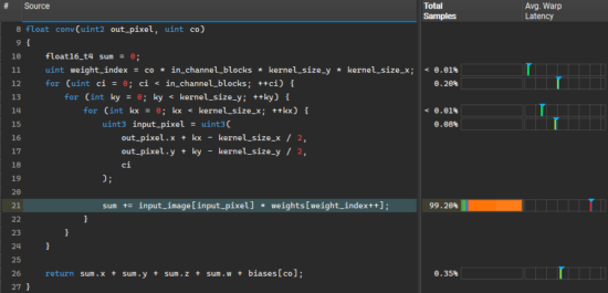
So that doesn’t help us very much, but we can look at the SPIR-V view to get some more information. Here we can see that most of the time is spent in reading the input image (OpImageRead), and the remaining time in the loading of the weights (OpLoad). In the stall attribution columns we can see these instructions wait either for a spot in the texture loading queue (texture throttle, TEXTHR) or wait for the data to arrive from global memory (long scoreboard, LGSB). In contrast, the multiplication and addition don’t have a single sample attributed to it.
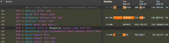
This makes it clear we should still focus on optimizing memory traffic before worrying about anything else.
Utilizing shared memory
One of the most powerful tricks in our toolbox to optimize memory traffic is utilizing shared memory. This is a small dedicated pool of memory physically located on each workgroup processor (Streaming Multiprocessor/SM on NVIDIA and Compute Unit/CU on AMD). It is much faster to access than global memory, but it is relatively small and contents is only shared with threads in the same workgroup.
In our current kernel every thread reads 9 pixels of each input channel. But the neighbouring threads also need some of those same pixels. Consider the following image where each square represents a pixel:
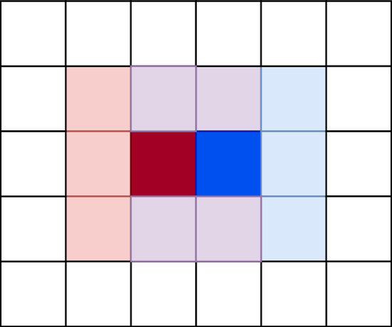
The threads for the red and blue pixels need local neighbourhood of pixels to calculate their results. This neighbourhood overlaps: in this image the red and blue pixels share 6 pixels in their respective neighbourhoods. When considering more than just these two neighboring pixels, every pixel is included a total of 9 times. So if we consider a 4×4 image tile, we get the following overlap counts:
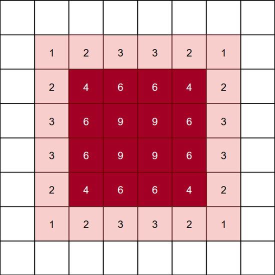
This is what we can optimize by using shared memory. We load all the image data required for calculating the 4×4 tile of pixels to shared memory once. For this example this is the dark red 4×4 tile and the additional one pixel border around all sides. After preloading, all the threads (16 in this example) can load the required input data directly from shared memory, thus wasting no time on duplicate loads.
Our implementation for this will consist of couple of parts. First, we must define our array of shared memory using the groupshared keyword. We’ll use a multidimensional array for easy indexing. We base the size of the input tile to load on the group size we defined for the kernel. So the larger the group, the larger the shared memory usage.
// Size of the input tile in group shared memory
// Equal to the local size xy, but with added padding on all sides
// Note that local_size_xy are specialization constants indicating the workgroup size
static const uint input_tile_width = local_size_x + kernel_size_x / 2 * 2;
static const uint input_tile_height = local_size_y + kernel_size_y / 2 * 2;
static const uint input_tile_size = input_tile_width * input_tile_height * in_channel_blocks;

// Tile of input data in shared memory
groupshared float16_t4 input_shared[in_channel_blocks][input_tile_height][input_tile_width];Next is the function that will take care of preloading input data to shared memory. We’ll have every thread in the group collaborate load data to maximize memory coalescing. So we’ll do a linear loop through the input window we want to load, where each thread individually determines the next element to load and store it in shared memory.
void preload_input(const uint2 input_offset, const uint thread_idx, const uint group_size) {
    // Linear thread-strided loop to load window
    for (uint wi = thread_idx; wi < input_tile_size; wi += group_size) {
        // Decompose 1D window index to window x, window y and input channel (block)
        const uint wx = wi % input_tile_width;
        const uint wy = (wi / input_tile_width) % input_tile_height;
        const uint ci = wi / (input_tile_width * input_tile_height);

        // Determine global pixel coordinate to load
        const int2 offset   = int2(wx - kernel_size_x / 2, wy - kernel_size_y / 2);
        const int3 in_pixel = int3(input_offset + offset, ci);

        input_shared[ci][wy][wx] = input_image[in_pixel];
    }
}Our main kernel entry point will also change a bit. The kernel now consists of two phases: the preloading and the actual convolution. Between the two phases we must make sure every thread in the workgroup has finished the previous phase using GroupMemoryBarrierWithGroupSync().
void main(
    uint3 dispatch_thread_id : SV_DispatchThreadID,
    uint3 group_id : SV_GroupID,
    uint3 thread_id : SV_GroupThreadID,
    uint thread_idx : SV_GroupIndex
) {
    // Preload input for the tile of pixels this workgroup governs
    const uint3 group_size = WorkgroupSize();
    const uint total_group_size = group_size.x * group_size.y * group_size.z;
    preload_input(group_id.xy * group_size.xy, thread_idx, total_group_size);

    // Wait for all threads to reach this point
    GroupMemoryBarrierWithGroupSync();

    // Loop through output channels, perform convolution for each channel
    for (uint co = 0; co < out_channel_blocks; ++co) {
        // ... loop contents remains the same ..
    }
}The final change we need is to make our conv() function load data from shared memory instead of global memory. This actually simplifies our index calculation. We can replace the inner loop with:
float16_t4 sum = 0;
for (uint ci = 0; ci < in_channel_blocks; ++ci) {
    for (int ky = 0; ky < kernel_size_y; ++ky) {
        for (int kx = 0; kx < kernel_size_x; ++kx) {
            // The shared memory array is already indexed in coordinates local to
            // our workgroup. So we can directly use the local thread id and
            // the kernel offset here.
            const uint2 window_id = thread_id.xy + uint2(kx, ky);
            sum += input_shared[ci][window_id.y][window_id.x] * weights[weight_index++];
        }
    }
}And with that we can run our new kernel. The improvements are pretty great: down to 74ms. A roughly 1.7x speedup compared to our previous result and 5.3x as fast of our original naive kernel.
| Naïve | 393ms |
| Packed vectors | 259ms |
| Conversion to fp16 | 124ms |
| Shared memory | 74ms |
| Target | 33ms |
Some notes on workgroup sizes
This is still using a workgroup size of 8x8x1. We might be able to get better results if we use a larger workgroup size, so that we get more pixel re-use. But this also increases our shared memory usage. If we use more shared memory, it means fewer workgroups can be scheduled concurrently on the same compute unit. This reduces the GPUs ability to improve performance by latency hiding: scheduling other warps while waiting for global memory loads to arrive.
For our workgroup of 8×8 pixels we current use a 10×10 tile of pixels. For 64 input channels and 2 bytes per fp16 element, this leads to 10 * 10 * 64 * 2 = 12.5KB of shared memory usage per workgroup. The Vulkan spec states at least 16KB of shared memory should be available on every Vulkan implementation. In practice, most devices have at least 32KB available (source). Below is a table indicating how much memory would be needed for various workgroup sizes.
| Workgroup X | Workgroup Y | Required shared memory (64 channels; 3×3 filter) |
| 8 | 8 | 12.5KB |
| 16 | 8 | 22.5KB |
| 16 | 16 | 40.5KB |
| 32 | 16 | 76.5KB |
| 32 | 32 | 144.5KB |
On my RTX 500 Ada I can use 49KB per workgroup. Meaning I could run this kernel with a 16×16 workgroup size. This provides a minor improvement over the 8×8 version (71ms), but there is another optimization we can do here.
We currently only utilize the X and Y dimensions of the workgroup, and every thread currently iterates over all output channels. But as the output for each channel is independent of other channels, we could utilize the Z dimension to parallelize over the output dimensions as well. Simply changing the output channel loop to take the index and size of the Z dimension allows us more freedom in determining how many threads we want per workgroup without increasing shared memory usage:
// Loop through output channels in a grid-strided loop
for (uint co = thread_id.z; co < out_channel_blocks; co += group_size.z) {
    // .. Same as before ..
}Now we can freely change the Z dimension of our workgroup size as well and see what works best. Some experimentation shows that on my specific GPU, 16x8x4 performs best. Reducing our kernel runtime to 68ms.
| Naïve | 393ms |
| Packed vectors | 259ms |
| Conversion to fp16 | 124ms |
| Shared memory (8x8x1) | 74ms |
| Shared memory (16x8x4) | 68ms |
| Target | 33ms |
Tweaking this workgroup size is definitely more an art than a science. The optimal value can depend on many hardware-specific factors. A proper production implementation would check the available memory at runtime, benchmark some configurations on-the-fly and select the best option automatically.
Wrapping up (for now)
Let’s wrap up by looking at an Nsight trace of our kernel again. With the latest version, all the kernel’s time is still spent on the sum += input * weight line, but now the stall reasons are very different. While previously our kernel spent most of its time in OpImageRead / OpLoad, now most of the samples land on OpFMul, with the top listed stall reasons being NOTSEL (Not Selected) and MATHTH (Math Pipe Throttle). The former indicates there are often warps ready to run which don’t run because of tied up resources, which has the same reason as our second stall: the math pipe. Our kernel is now limited by computational load rather than memory traffic.
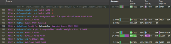
This is directly visible in the SM throughput, which increased to 85%. This means we are getting closer to the “speed-of-light” of my GPU. Once we reach that, improvements will have to come from some other tricks. But as this post is getting somewhat long already, I’ll get back to those in the next part!
For now, I hope you enjoyed this write up. In the meantime, if you have a GPU workload that doesn’t quite give you the performance you’d like we would love to hear from you!
References
[1] Lehmann, Moritz, et al. “Accuracy and performance of the lattice Boltzmann method with 64-bit, 32-bit, and customized 16-bit number formats.” Physical Review E 106.1 (2022).