
In the world of high-performance programming, true portable code has been a goal for a long time. Vulkan has been very successful at this, with Vulkan drivers being provided by every major GPU vendor and available for all common desktop and mobile operating systems. Platforms without first party support (e.g. Apple macOS/iOS) have compatibility layers available that seamlessly make everything work regardless.
At Stream HPC, we have been using Vulkan for the last few years for any problem that requires portability. So much so that we have been building a library to streamline the use of Vulkan for HPC applications. As part of our library we’re been implementing a set of example compute problems you can solve with Vulkan.
In this blog post we will detail the implementation of one of these examples: neural upscaling using convolutional networks. We’ll briefly introduce how convolutional neural networks work, but will mostly focus on how to implement those in Vulkan compute shaders. We’ll also be leaving out some of the Vulkan scaffolding necessary to make this a full standalone application. There’s some great guides available for that already.
Neural upscaling
Many neural methods exist to upscale images from lower resolution to higher resolutions. Over the last years it has seen extensive use in games and image processing applications. To keep the scope of this example manageable we’ll use a technique from 2016, introduced in “Real-Time Single Image and Video Super-Resolution Using an Efficient Sub-Pixel Convolutional Neural Network” [1].
The technique makes use of convolutional neural networks (CNN), the ubiquitous technique for neural image processing.
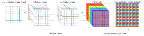
The super-resolution network architecture is simple: 4 consecutive 2D convolution layers. All layers have a stride of (1, 1) and a padding of half the kernel size (rounded down). This configuration makes every layer output an image of the same size, so no up- or down-convolution is happening.
Below, the full architecture is listed. Note that the output channels of the last layer are dependent on the desired upscale factor. So when upscaling an image 300%, you’ll end up with 9 output channels.
# channels in, channels out, kernel size
conv1 = conv2d(1, 64, (5, 5))
conv2 = conv2d(64, 64, (3, 3))
conv3 = conv2d(64, 32, (3, 3))
conv4 = conv2d(32, upscale_factor**2, (3, 3))

def forward(x):
    x = relu(conv1(x))
    x = relu(conv2(x))
    x = relu(conv3(x))
    x = conv4(x)

return xAs you can see the network only has a single input channel. This is the luminance component the input pixels. To upscale an RGB image, it first must be converted to YCbCr color space. The luminance is then upscaled using the neural method, while the blue and red chroma components are upscaled using simple bilinear or bicubic interpolation. This works because our eyes are less sensitive to color changes than luminance changes. In fact, this method goes back all the way the first analog video transmissions for color TV and is still used in most modern compressed digital media formats (see chroma subsampling for more information).
Also note that each layer (except for the last layer) is followed by a ReLU function. This is the activation function, which are sometimes called the “non-linearity”. They are essential components of deep neural networks, as they make it possible for the network to express a non-linear function. The presence of this activation function will be important when implementing our convolution kernel.
After feeding the image through the convolutional network you will end up with a similar sized network, but with more output channels. Each of these output channels represents a “sub-pixel” in the upscaled image. To retrieve the final upscaled image, the channels must simply be reshuffled where 9 channels form a 3×3 output block (i.e. reshuffle each 1x1x9 block to 3x3x1).
Loading an ONNX model
For this example we are not too interested in training the network. So we’ll use a pretrained ONNX model available from the ONNX model repository. These models can be loaded using the ONNX library.
It is important to know that ONNX models are internally just Protocol Buffers. This means that as long as we have the generated definitions for our language of choice, we don’t actually need the entire ONNX library.
In our case, we just build the ONNX library once, grab the generated C++ definitions and use only protobuf (lite) at runtime. Or instead of building the ONNX library you can also download the ONNX protobuffer definitions (*.proto3 files) and run them through the protobuffer compiler yourself. Either way you should end up with onnx.pb.h and onnx.pb.cc which you can just include in your project.
Loading the model then looks like this:
onnx::ModelProto load_model(std::string_view path) {
    onnx::ModelProto onnx;

    size_t size;
    std::byte[] data = load_file(path, &size);

    if (!data)
        throw std::runtime_error("Failed to open ONNX file");

    if (!onnx.ParseFromArray(data, static_cast<int>(size)))
        throw std::runtime_error("Failed to parse ONNX model");

    return onnx;
}We could use this model file to build the model graph dynamically (i.e. all the computational steps needed for the model). The model graph can be retrieved using onnx::ModelProto::graph(). This returns a GraphProto object, whose graph nodes can be enumerated using onnx::GraphProto::node().
But for now we’ll just hard-code our graph based on the paper and only load the corresponding weights for each pass. Weights and biases are stored in the graphs “initializer” tensors, which can be accessed using onnx::GraphProto::initializer(). We can retrieve the values from the tensors as follows:
// Helper function to find a named tensor
const onnx::TensorProto* find_tensor(const onnx::ModelProto& onnx, std::string_view name) {
    for (const auto& tensor : onnx.graph().initializer()) {
        if (tensor.name() == name)
            return &tensor;
    }

    return nullptr;
}

std::vector<float> tensor_values(const onnx::ModelProto& onnx, std::string_view name) {
    // Find tensor by name
    const onnx::TensorProto* tensor = find_tensor(name);
    if (!tensor) {
       throw std::logic_error("Weights named {} not found in model", name);
    }

    // Validate data type
    const auto type = static_cast<onnx::TensorProto_DataType>(tensor->data_type());
    if (type != onnx::TensorProto_DataType_FLOAT) {
        throw std::logic_error("Tensor has unsupported data type (Only FP32 is supported)");
    }

    // Copy raw data to a float vector
    const auto& raw_data = tensor->raw_data();
    size_t      count    = raw_data.size() / sizeof(float);

    std::vector<float> data_list(count);
    std::memcpy(data_list.data(), raw_data.data(), raw_data.size());

    return data_list;
}In the linked ONNX file the tensors are named conv1.weight, conv1.bias, conv2.weight, etc. For the weights we expect one kernel per combination of input and output channel, so we get input channels * output channels * kernel width * kernel height weights per layer. The biases we just have one per output channel, so just output channels bias values per layer.
It is also important to note that while network has been trained of images of size 224×224 pixels, it is in fact “fully convolutional”. Which means that it doesn’t have any fully connected linear layers or other elements that would force it to work with a fixed input size. As the convolution operation is applied per-pixel, we can simply apply it to input images of any size and get back an upscaled output image (but the results will be best when images match the training size).
Now we need to upload those to GPU memory for use in our convolution kernel. Vulkan offers two types of generic buffer memory: storage buffers (SSBO) and uniform buffers (UBO). Uniform buffers are read-only and usually have dedicated hardware caching mechanisms. That would in theory be ideal for our static weights and biases, but most devices only support uniform buffers up to 64KB (source). You’d already exceed this limit with a 5×5 kernel for 32 input and output channels. So we’ll use storage buffers instead.
Now we can just load the weights and biases for each layer and start doing convolution!
The convolution kernel
Now that we loaded weights we can start work on our convolution kernel. The general form for calculating the updated value for a pixel at and output channel is:

A very naïve implementation requires 4 nested for-loops to run this equation for each output channel. This is easily parallelized by running each thread on a different pixel (in fact, it is a typical example of an “Embarrasingly Parallel” problem). Let’s first implement this naïve kernel and get our pipeline working, we can look at optimizations later.
For Vulkan we need to write this kernel in a language to compile to SPIR-V bytecode. We use the Slang language for writing shaders. It makes our kernel looks something like this:
void main(uint3 dispatch_thread_id : SV_DispatchThreadID) {
    const uint2 out_pixel = uint2(dispatch_thread_id.xy);

    // Loop through output channels, perform convolution for each channel
    // (Unoptimized just for demonstration purposes, not suitable for real use)
    uint weight_index = 0;
    for (uint co = 0; co < out_channels; ++co) {
        float sum = 0;
        for (uint ci = 0; ci < in_channels; ++ci) {
            [[unroll]]
            for (uint ky = 0; ky < kernel_size_y; ++ky) {
                [[unroll]]
                for (uint kx = 0; kx < kernel_size_x; ++kx) {
                    // Determine coordinate of input pixel to read
                    uint3 input_pixel = uint3(
                        out_pixel.x + kx - kernel_size_x / 2,
                        out_pixel.y + ky - kernel_size_y / 2,
                        ci
                    );

                    // Apply convolution weight
                    sum += input_image[input_pixel] * weights[weight_index++];
                }
            }
        }

        // Add bias
        float result = sum + biases[co];

        // Apply ReLU (if needed) and write output
        output_image[uint3(out_pixel, co)] = apply_relu ? relu(result) : result;
    }
}
(Note that range checks and binding definitions have been excluded for clarity.)
Bindings
Below we list the bindings needed for the input and output data of our convolution kernel. As said, we store our weights and biases in storage buffers. Which in Slang we map to StructuredBuffer<T>, allowing us to index them as arrays.
StructuredBuffer<float> weights, biases;

RWTexture3D<float> input_image, output_image;We also define our input and output images as RWTexture3D<T>. Mapping these to 3D textures makes for slightly easier indexing using the channel as the Z-coordinate. Textures can also be stored more optimally for accessing neighboring pixels (when created with tiling mode VK_IMAGE_TILING_OPTIMAL).
But as always, that’s all theoretical and in practice there can be many implementation differences between different hardware. This benchmark shows how it is very hardware dependent and it’s very difficult to decide on what’s optimal everywhere without measuring: https://github.com/sebbbi/perftest.
Specialization constants
In our kernel above you can see that per output channel we also (conditionally) apply the ReLU function. We could do this in a separate pass which we schedule conditionally, but that would just cause a bunch of extra memory traffic which we don’t want.
In order to make sure the conditional disappears in the final kernel, we use a specialization constant to set the apply_relu value. This gives us basically two variants of the kernel: one that applies ReLU and one which doesn’t.
We also use specialization constants for setting the kernel size (kernel_size_x / kernel_size_y). This allows the SPIR-V compiler to unroll the inner two loops based on the exact kernel size without having to add runtime bounds checks.
The full of specialization constants and bindings are listed below:
[[SpecializationConstant]]
const int kernel_size_x, kernel_size_y;

[[SpecializationConstant]]
const int out_channels, in_channels;

[[SpecializationConstant]]
const bool apply_relu = true;The values for these specialization constants need to be specified when creating the compute pipeline in the Vulkan API (as part of your parameters of vkCreateComputePipelines()). The downside of this is that you do need to create a different pipeline for each combination of specialization constants you want to use. In our case, every CNN layer has a unique combination of specialization constants, so we can just create 4 pipelines.
In order to properly define the mapping from your specialization data to the layout the kernel expects, you need to know the “specialization constant ID” of each constant. You can either manually specify those in Slang by using the [vk:constant_id(id)] attribute (See the docs) or use SPIRV-Reflect to reflect the automatically generated layout from the SPIR-V code. Once you know constant IDs, you can set their values as follows:
// Create specialization map with 3 uint32 entries
// (We're skipping out_channels/in_channels here for simplicity)
VkSpecializationMapEntry entries[] = {
    {
        .constantID = 0,
        .offset = 0,
        .size = sizeof(uint32_t)
    },
    {
        .constantID = 1,
        .offset = sizeof(uint32_t),
        .size = sizeof(uint32_t)
    },
    {
        .constantID = 2,
        .offset = sizeof(uint32_t)*2,
        .size = sizeof(uint32_t)
    }
};

// Values to bind to the spec constants (kernel_size_x, kernel_size_y, apply_relu)
uint32_t values[] = { 3, 3, 1 };

VkSpecializationInfo spec_info = {
    .mapEntryCount = 3,
    .pMapEntries = &entries,
    .dataSize = sizeof(uint32_t) * 3,
    .pData = values
};

// Add the spec info to the pipeline creation info
VkComputePipelineCreateInfo pipeline_info{
    // ...
    .stage = {
        // ...
        .pSpecializationInfo = &spec_info
    }
};

// Create the actual pipeline
VkPipeline pipeline;
vkCreateComputePipelines(device, nullptr, 1, &pipeline_info, nullptr, &pipeline);(Note that we simplified our value list a bit by also considering apply_relu a uint32_t value. This works because boolean values are 32-bit in Vulkan)
If this looks like a lot of work, this is exactly where our Vulkan Compute library would help out! For reference, in our library this entire block can be replaced by:
auto kernel = vkc::Kernel(spirv, {
    { "kernel_size_x", 3 },
    { "kernel_size_y", 3 },
    { "apply_relu", true },
});Dispatching kernels
In Vulkan, if you want to dispatch a Kernel you usually add it to a command buffer using a combination of vkBindPipeline()(to bind your previously created pipeline) and vkCmdDispatch() (to specify the number of compute work groups i.e. block count to launch). If you come from a CUDA or HIP background it might surprise you that while you can specify your group count, you can’t set your group size! Instead, this must be specified in the shader itself. In Slang, you’d use the [[numthreads]] attribute on your kernel entry point. Making it look something like this:
[[numthreads(8, 8, 1)]]
void main(uint3 dispatch_thread_id : SV_DispatchThreadID)
{
    // ...
}This has a couple of downsides: you must manually synchronize this value with your host code to make sure you dispatch the correct number of groups and you can’t optimize the group size for the specific hardware your shader runs on.
But there’s a neat trick here that can help us. You can set this value using specialization constants. That allows us to specify the group size from the host code, keeping the values in sync and allows us to implement custom logic for determining the optimal group size.
We’ve shown how to set specialization constants in the previous chapter, but here again the code becomes much nicer with our Vulkan Compute library. Here’s an example:
// In your Slang shader:
__vkc_kernel__ void main(uint3 dispatch_thread_id : SV_DispatchThreadID)
{
    // ...
}

// In your C++ host code:
const auto group_size = vkc::KernelGroupSize(8, 8, 1);
auto kernel = vkc::Kernel(spirv, { /* other spec constants */ }, group_size});

// Dispatch kernel. Base number of groups on the image size and selected group size
kernel.dispatch(command_buffer, vkc::group_count(input_image, group_size));This also allows us to automatically try out various group sizes to select the most performant configuration on-the-fly.
Putting it together
Before we can upscale an image, we need two more kernels:
- A “encode” kernel to convert the input RGB image to separate Y, Cb and Cr images.
- A “decode” kernel to perform the channel shuffle which converts the 9-channel output of the CNN to a 3x upscaled image, and converts back to RGB.
We could use the VK_KHR_sampler_ycbcr Vulkan extension to skip having to implement the YCbCr to RGB conversion ourselves. However, the opposite direction is not supported (there’s VK_VALVE_video_encode_rgb_conversion but it’s very new and available on very few implementations) and conversion between RGB and YCbCr is fairly trivial. So instead we’ll be using the formulas taken from this neat reference page. This maps nicely to a 3×3 matrix multiplication. Here’s a small kernel to do the encoding:
RWTexture2D<float4> in_rgb;

RWTexture3D<float> out_y;

RWTexture2D<float> out_cb, out_cr;

static const float3x3 rgb_to_ycbcr = float3x3(
    0.299,  0.5870,  0.1140,
   -0.167, -0.3313,  0.5000,
    0.500, -0.4187, -0.0813
);

void main(uint3 dispatch_thread_id : SV_DispatchThreadID) {
    const uint2 pixel = uint2(dispatch_thread_id.xy);

    // Convert RGB to YCbCr
    const float3 ycbcr = mul(rgb_to_ycbcr, in_rgb[pixel].rgb);

    // Write output
    out_y[uint3(pixel, 0)] = saturate(ycbcr.x);

    out_cb[pixel] = saturate(ycbcr.y + 0.5);
    out_cr[pixel] = saturate(ycbcr.z + 0.5);
}(Note that out_y is a 3D texture as this is used as input for our convolution kernel)
Decoding is a little bit more complicated, but not by much. Besides the conversion back to RGB it also contains the channel shuffle. Here’s the full kernel:
RWTexture2D<float4> out_rgb;

RWTexture3D<float> in_y;

Sampler2D<float> in_cb, in_cr;

static const float3x3 ycbcr_to_rgb = float3x3(
      1.0,  0.00000,  1.40200,
      1.0, -0.34414, -0.71414,
      1.0,  1.77200,  0.00000
);

void main(uint3 dispatch_thread_id : SV_DispatchThreadID) {
    const uint2 out_pixel = uint2(dispatch_thread_id.xy);

    const uint2  in_pixel = uint2(out_pixel / 3);
    const float2 in_uv    = out_pixel / float2(out_width - 1, out_height - 1);

    // Get Y channel from a 3x3 block of channels
    const uint y_channel = (out_pixel.y % 3) * 3 + (out_pixel.x % 3);

    // Read the correct Y value
    const float y = in_y[uint3(in_pixel, y_channel)];

    // Sample Cb/Cr
    const float cb = in_cb.SampleLevel(in_uv, 0) - 0.5;
    const float cr = in_cr.SampleLevel(in_uv, 0) - 0.5;

    // Convert back Y, Cb and Cr to RGB
    const float3 rgb = mul(ycbcr_to_rgb, float3(y, cb, cr));

    // Write output
    out_rgb[out_pixel] = float4(saturate(rgb), 1.0);
}(Note that in_cb and in_cr are samplers instead of storage textures. This allows us to use hardware bilinear / bicubic sampling. in_y is just the output texture from the last convolution pass.)
After decoding we get back our upscaled RGB image for our viewing pleasure. Let’s take a look at the result.
Results
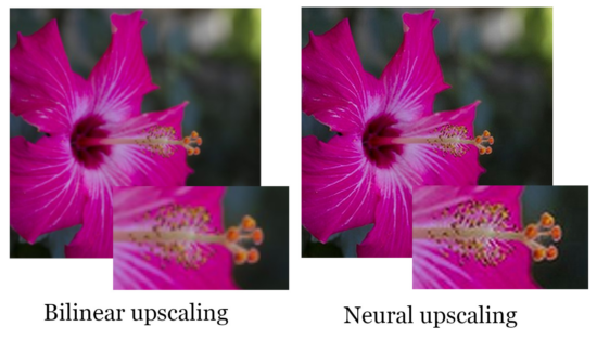
To test our new model, we run it on a test image downscaled to the original training resolution of 224×224 pixels. Below is the result with some details highlighted. We can see that the neural model is definitely better at enhancing some of the finer details.
But were you to zoom in a bit you will notice some artifacts in the neural upscaling. Around the anther there are some blocky artifacts and near the edges of the petals we get a halo effect. Nevertheless, this is a decent result for a technique from 2016 with a very simple network!
Performance
On my RTX 500 laptop GPU the entire CNN for this 224×224 image runs in 22ms. Not bad, but that’s a tiny image. For an 1280×720 image this is about 430ms. Which is pretty slow if we want to do this upscaling in real-time. Even with a 30fps video source, we would need to run in less than 33ms and thus it would need to be about 13 times as fast!
But don’t worry, there’s a bunch of optimization we can do to this convolution kernel to make it a lot faster. We’ll look into packing values for vectorized load and math instructions, utilize shared memory for reducing memory pressure, and look into specialized alternative convolution algorithms. These optimizations will result in a more than 10x speed increase and bring us very close to our target.
Those will be topics for next time though! For now, we hope you enjoyed this post.
Do you also have a compute problem you want solved anywhere on all devices? Don’t hesitate to contact us!
References
[1]: Shi, Wenzhe, et al. “Real-time single image and video super-resolution using an efficient sub-pixel convolutional neural network.” Proceedings of the IEEE conference on computer vision and pattern recognition. 2016.
[2]: Rawzor. “The New Test Images”: https://imagecompression.info/test_images/.