
The times before the advent of compute shaders, twenty years ago, were heroic. GPU came out of infancy into adolescence: the pace of innovation was breathtaking. A year without new GPU architecture was unthinkable. You could see new programming languages and APIs appearing one after another, bringing us closer and closer to “real-time photorealistic rendering” (by the standards of 2005, of course :)). And imaginative researchers started to explore the idea of using this power for general-purpose computation. In this post, we’re going to recall how calculations were implemented using OpenGL back then, because compute shaders were introduced only in OpenGL 4.3 in 2012 – much later than CUDA and even OpenCL. Before that, there were several hacks and workarounds to use GPUs for general-purpose computation. Let’s consider the “heroic” times and how it was done back then.
N-body problem
The exemplary problem that allows many parallel processors to demonstrate their advantages is N-body simulations in astrophysics. Naive approach includes calculation of all pairwise forces between bodies, that results in complexity. Even if the Newton force (with regularization) is as simple as , with – that is not even a galaxy, just a globular cluster – this means about operations per step which is not very feasible even on a modern CPU, let alone Pentium 4 that was the state of the art back then. The approaches to reduce that complexity are of course known, including octree-based algorithms like Barnes-Hut, hierarchical and multipole modelling and adaptive mesh refinement – all them come to nearly . But even in those algorithms force calculations bottlenecked the performance so much that Japanese astrophysicists developed specialized **hardware** called GRAvity PipE (GRAPE) to compute in parallel pairwise interactions. That thing beats all of general-purpose and super-computers by orders of magnitude from 1990 till the middle of 2000s (of course, only on gravitational force evaluations). I would love to talk about that, but that’s another story.
The fact that each force can be computed independently given positions of all bodies, makes this problem perfectly suited for GPUs, and it was realized quickly. Early GPUs had fixed computational pipeline not suited for anything besides rasterization, but with the introduction of vertex and fragment shaders it became possible to use GPUs for more than just graphics.
Instruments of the stone age
The first true programmability of compute pipeline arrived with the DirectX 8 generation of graphics cards in 2001: NVIDIA Geforce 3 and ATI Radeon R200. From OpenGL it was first exposed via vendor-specific extensions such as NV_vertex_program and ATI’s EXT_vertex_shader, but soon – in the next year – it was promoted to the multi-vendor ARB_vertex_program (eh, really heroic pace, now only AI-related things are developing so fast). This extension allowed full control over the vertex transformation pipeline, that later was joined by pixel/fragment transformations. At first it was still very limited, for example in Microsoft’s pixel shader (or fragment program/function/shader, in OpenGL terms) of version 1.1 the maximum number of texture fetch instructions was 4, and the maximum number of arithmetic instructions was 8 – with no branching allowed, of course. But each new version relaxed these limits substantially (branching appears in 2004 in 3.0), and by the time of 4.0 version in 2006 the rigid instruction-count limits of the earlier models had largely disappeared.
OpenGL was not designed for GPGPU, being graphics-oriented API. So for the computational applications people developed several higher-level approaches with more computation-oriented API. The most famous of those languages were NVIDIA’s Cg (it was essentially early HLSL in disguise), and Stanford University graphics group’s BrookGPU. Both were used to demonstrate possibility to roll out the N-body simulations to GPU.
The first bird
In 2004, Lars Nyland, Mark Harris, and Jan Prins from University of North Carolina at Chapel Hill applied Cg to run N-body simulation using fragment shaders – now and then computational power of that GPU part was much better than that of vertex pipelines. You cannot simply find out their paper on the Internet, but a curious reader can check the later technical report and recollections in section 31.5 of GPU Gems 3.
Many obstacles were overcome to run N-body simulation using OpenGL in 2004 – even a simple brute-force approach developed by them was not a trivial task, recalling the fundamental limitation that buffers were only read-only or write-only. The bodies were stored as a standard RGBA floating-point texture. The RGB channels were mapped to the body’s position, and the A channel was used to store its mass. For the force calculation, the quad was rendered into a force texture of by a Cg fragment program and a lookup texture to find corresponding and (yes, there was no blockIdx and threadIdx at that time). Total force on each body was found by parallel log reduction of , each step of reduction was rendering a quad of half the height of the previous one. This was severely bandwidth bound, because there was no shared memory on the GPU available from Cg. Finally, other fragment programs updated velocity texture and position texture with a single time step value over all the system. The number of bodies per single simulation block was limited by – it was the maximum allowed texture size on a GeForce flagship 6800 card. But it was still three times faster than the same-scheme CPU implementation. Later, this implementation was extended to work on many body chunks in parallel over a single GPU and cluster nodes, with reported performance of about calculated pair interactions per second on a 7 nodes cluster.
ATI strikes back
ATI side followed slightly later – the techreport above says that GeForce 6800 was chosen because ATI flagship Radeon X800 XT supported only 24-bit floating point calculations and not full f32 ones. Next generation of ATI chips R500 lifted that limitation, and in 2006 a group at Stanford University used the BrookGPU to run N-body on ATI X1900 XTX GPU (my first really 3D-accelerating GPU, by the way). Basically the same scheme was used in their calculations, besides that each pixel summed all the pairwise forces in a single shader – instruction count limits already improved by that time. They compared their GPU performance to a state-of-the-art CPU implementation in SSE assembly and found a factor of 25 speedup over Pentium 4 – 100 GFLOPS vs 4 GFLOPS, to be precise.
GPU came to state-of-the-art N-body
But it was still not enough to beat GRAPE hardware, and the implementations were mainly proof-of-concept rather than serious applications – the first implementation of the state-of-the-art N-body simulation on GPU appears in 2007 and on GeForce 8800GTX it was still ~8 times slower than GRAPE-6Af up to the point where particle data size exceed GRAPE memory limit. To give you a taste of the code of this implementation, here’s the calculation kernel written in Cg:
void compute_acc_jerk_and_pot(
    in float2 coords : TEXCOORD0,          // 2D texture coordinate of this particle
    out float3 acc : COLOR0,               // Output texture with acceleration
    out float4 jerkAndPot : COLOR1,        // Output texture with jerk and potential
    uniform samplerRECT accTexture,        // Input texture with all particles’ acceleration
    uniform samplerRECT jerkAndPotTexture, // ,, ,, ,, ,, ,, jerk and potential
    uniform samplerRECT massTexture,       // ,, ,, ,, ,, ,, mass
    uniform samplerRECT posTexture,        // ,, ,, ,, ,, ,, position
    uniform samplerRECT velTexture,        // ,, ,, ,, ,, ,, velocity
    uniform float eps2,                    // Softening parameter
    uniform float otherParticle,           // Index to other particle
    uniform float texSizeX,                // Width of all textures
    uniform float texSizeY,                // Height of all textures
    uniform float offset )                 // Number of unused texture elements
{
    float  coords1D, newCoords1D, otherMass,
           r2, xdotv, r2inv, rinv, r3inv, r5inv, xdotvr5inv;
    float2 newCoords;
    float3 pos, otherPos, vel, otherVel, dx, dv, thisAcc, thisJerkAndPot;

    // Get data from the textures
    acc        = texRECT(accTexture, coords).rgb;
    jerkAndPot = texRECT(jerkAndPotTexture, coords).rgba;
    pos        = texRECT(posTexture, coords).rgb;
    vel        = texRECT(velTexture, coords).rgb;

    // Convert the 2D texture coordinate to 1D and increase with otherParticle
    // to obtain the coordinate of this iteration’s other particle. Because our
    // textures are defined as samplerRECT, texture elements must be addressed
    // as (x+0.5,y+0.5). When converting to 1D, we must compensate for this offset).
    coords1D    = round(coords.y-0.5) * texSizeX + round(coords.x-0.5);
    newCoords1D = coords1D + otherParticle;

    // Skip over unused texture elements
    if (newCoords1D + offset > texSizeX*texSizeY - 1)
        newCoords1D = newCoords1D - (texSizeX*texSizeY - offset);

    // Convert the other particle’s 1D coordinate to 2D. As above, we must add
    // 0.5 to obtain correct texture element coordinates.
    newCoords = 0.5 + float2( frac(newCoords1D/texSizeX)*texSizeX,
                              floor(newCoords1D/texSizeX) );

    // Get the position, velocity and mass of this iteration’s other particle
    otherPos  = texRECT(posTexture, newCoords).rgb;
    otherVel  = texRECT(velTexture, newCoords).rgb;
    otherMass = texRECT(massTexture, newCoords).r;

    // Compute acceleration, jerk and potential
    dx = otherPos-pos;
    dv = otherVel-vel;
    r2 = eps2 + dot(dx,dx);
    xdotv = dot(dx,dv);
    r2inv = 1.0/r2;
    rinv = sqrt(r2inv);
    r3inv = r2inv*rinv;
    r5inv = r2inv*r3inv;
    xdotvr5inv = 3.0*xdotv*r5inv;
    thisAcc = otherMass*r3inv*dx;
    thisJerkAndPot = otherMass*(r3inv*dv - xdotvr5inv * dx);
    acc = acc + thisAcc;
    jerkAndPot.rgb = jerkAndPot.rgb + thisJerkAndPot;
    jerkAndPot.a = jerkAndPot.a - otherMass*rinv;
}First interesting part is the size and number of parameters, more typical for graphics applications like Vulkan, rather than computational CUDA/HIP/SYCL ones. Second part worth paying attention to is coordinate handling here through textures. Although the implementation used GPU only to calculate forces on individual particles, this was still unavoidable. Integration of the system itself was done on CPU with a fourth-order Hermite predictor-corrector integrator with block time steps – that was made it the state-of-the-art N-body.
The new dawn: CUDA
The second paper of the series from the same University of Amsterdam group (only 5 months later) already celebrated CUDA and shared memory support – and the same GeForce 8800GTX GPU symbolically overcame GRAPE even at 1024 particles simulation (where hardwired on-chip GRAPE memory was enough). The following years show incredible developments in using both professional and consumer GPUs for scientific computing, and several Gordon Bell prizes on performance per dollar were awarded to the teams constructing these machines like shown here.
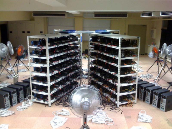
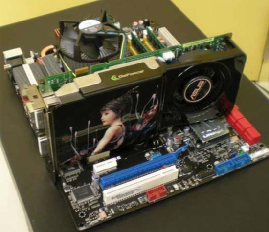
Left: 42 TFlops computer for N-body simulations of 2009 – 128 host PCs with 256 GPUs – a mining farm before it becomes mainstream :). And right its single node disassembled: CoreTM 2-Quad 2.4-GHz Q6600 processor on an X38 chipset motherboard with 2 NVIDIA GeForce 8800 GTS GPUs – landmark “girls on the GPUs” era.
Source: Hamada, Tsuyoshi and Narumi, Tetsu and Yokota, Rio and Yasuoka, Kenji and Nitadori, Keigo and Taiji, Makoto. 42 TFlops hierarchical N-body simulations on GPUs with applications in both astrophysics and turbulence (2009) Proceedings of the Conference on High Performance Computing Networking, Storage and Analysis.
Conclusion
And so the heroic era of scientific GPU computing through APIs never designed for it faded away. Over the following years came a steady flow of major GPU-computing APIs and programming models – OpenCL, DirectCompute/D3D11, OpenGL compute shaders, HIP, SYCL, and others – each of them making general-purpose GPU programming easier and more powerful.